IFFP Wiki
Hillslope Linkage Model (HLM)
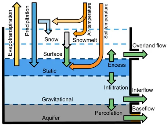
We simulate streamflow with the TETIS version of the Hillslope-Link Model (HLM) developed by the Iowa Flood Center (IFC) as discussed in Quintero and Velasquez (2022). The theoretical background and conceptualization of the HLM is comprehensively described in Mantilla et al. (2022). The TETIS version of HLM is a fully distributed hydrologic model structure, which is based on the decomposition of the landscape into hillslopes and channels. The model estimates runoff generation at the hillslope by simulating different processes Snow accumulation and melting rates are derived from precipitation and temperature data, based on the degree-day method. The model simulates precipitation losses in vegetation and soil pore macrostructure. Surface infiltration takes into account the hydraulic soil properties of the hillslope, and the conditions of frozen ground during the cold season. Deep percolation and groundwater losses are also modelled, considering the hydraulic conductivity of soil at the subsurface. Total hillslope runoff is aggregated in the river channel from the contribution of overland flow, interflow, and base flow. A nonlinear hydrologic routing model transports flow in the channels and takes into account the geomorphologic characteristics of the river network. The model equations are written as ordinary differential equations. HLM integrates a numerical solver that takes benefit of the binary tree structure of the river network to solve the system of differential equations in an asynchronous manner, suitable for high performance computing environments (Small et al., 2013). In our implementation, the HLM outputs streamflow simulations produced at an hourly time step, and annual maximum discharge is obtained for all channel links in the river network. Projections of precipitation, temperature, evapotranspiration, and frozen ground conditions are used as forcings into the hydrologic model. The spatial and temporal resolution of these inputs are key for the performance of the model (see Quintero and Velasquez (2022) for more details). Simulations are conducted under naturalized flow conditions where stream regulation (i.e., dams) is ignored due to the lack of available data on future operating procedures.
Future Projection Inputs
The web tools utilize climate model forcings from models part of the Coupled Model Intercomparison Project Phase 5 (CMIP5) and Phase 6 (CMIP6). CMIP6 are the results utilized on the main page.
CMIP5
IFFP utilizes precipitation, temperature, and evapotranspiration data from 19 of the Coupled Model Intercomparison Project 5 (CMIP5) global climate models (GCMs) (see Taylor et al. (2012) for more details) to generate streamflow projections. The CMIP5 daily climate projections simulations were downscaled statistically using bias-correction constructed analogues (BCCA; Maurer et al., 2010). The horizontal resolution of data is 1/8° latitude-longitude (~ 12km by 12 km). IFFP incorporates outputs for two emission scenarios or representative concentration pathways the emissions scenarios of (RCPs) (see Figure 1)RCP4.5 and RCP8.5.: 1) RCP4.5 is an intermediate emissions scenario where the peak emission occurs around 2040 and then declines; .2) RCP8.5 is an emission scenario in which emissions continue to rise throughout the 21st century. This provides robust coverage of projections to better prepare water resource management in the future. While we use 19 models (see below), they do not all perform equally. Based on Michalek et al. (2022), we have preselected a subset of the better-performing ones and identified them with (“*” below) as shown below.
The following are the GCMs used in the website:
- access1-0*
- canesm2
- cmcc-cm*
- cnrm-cm5*
- csiro-mk3-6-0*
- gfdl-cm3
- gfdl-esm2g
- gfdl-esm2m*
- hadgem2-cc
- hadgem2-es*
- inmcm4
- ipsl-cm5a-mr
- miroc5*
- miroc-esm*
- miroc-esm-chem
- mpi-esm-lr*
- mpi-esm-mr
- mri-cgcm3
- noresm1-m

CMIP6
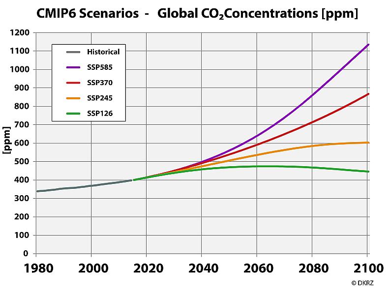
The web tool provides projections based on CMIP6 precipitation, temperature, and evapotranspiration data from 18 GCMs (see Erying et al. (2016) for more details). The CMIP6 daily precipitation climate projections simulations were downscaled statistically using quantile mapping. The horizontal resolution of data is 1/16° latitude-longitude (~ 4km by 4km). CMIP6 represents emission scenarios with shared socioeconomic pathways (SSPs). Figure 2 shows what each scenario represents in terms of SSPs. We utilize three scenarios (SSP245, SSP370, and SSP585) to provide robust coverage of projections to better prepare water resource management in the future. Based on Michalek et al. (2023), all 18 models provided perform well and all are utilized in the main IFFP page results.
The following are the GCMs in this web tool:
- access-cm2
- access-esm1-5
- canesm5
- cmcc-cm2-sr5
- cmcc-esm2
- ec-earth3
- ec-earth3-veg
- ec-earth3-veg-lr
- fgoals-g3
- gfdl-esm4
- iitm-esm
- inm-cm5-0
- kace-1-0-g
- miroc6
- mpi-esm1-2-hr
- mpi-esm1-2-lr
- mri-esm2-0
- taiesm1
Nonstationarity and flood peak estimates
Climate change presents a significant challenge to water resource engineers and planners as it will increase the likelihood of hydrometeorological extremes such as extreme precipitation and temperature (see AR6 IPCC 2021 Report for more details) . For many watersheds within Iowa this means that the annual maximum discharges are expected to increase over time creating a nonstationarity component. Current guidelines established by the United States Army Corps of Engineers (USACE) and the United States Geological Survey (USGS) for flood frequency analysis (see Bulletin 17C and Eash et al. (2012)) do not provide recommendations on how to account for climate change. This highlights a need for new guidelines and tools. For the main IFFP page, we fit a generalized extreme value distribution below with the nonstationarity assessed based on the Mann Kendall trend test.
Non-Stationarity Assessment
The presence of non-stationarity in a given record (simulated or observed) is analyzed by the non-parametric Mann-Kendall test. Given a dataset X consisting of x values with sample size n, the MK calculation starts by estimating the S statistic:
$$ {S=\sum^{n-1}_{i=1}\sum^{n}_{j=i+1}sign(x_j-x_i)}$$ where
$$ {sign = \begin{Bmatrix}1, & x_j>x_i\\0, & x_j=x_i\\-1, & x_j< x_i\end{Bmatrix}}$$ As indicated in Kendall (1975) when n ≥ 10 the distribution of S approaches the Gaussian form with mean E(S) = 0 and variance V(S) given by: $${ V(S) = \frac{n(n-1)(2n+5)-\sum^{m}_{j=1}t_jj(j-1)(2j+5)}{18}}$$ where tj is the number of ties of length m.
The statistic S is then standardized resulting in the MK final value. The significance of the MK statistic can be estimated from the normal cumulative distribution function (Z). Positive (negative) MK values indicate the presence of increasing (decreasing) trends. $${Z = \begin{Bmatrix} (S-1)/\sigma, & S>0\\0, & S=0\\(S+1)/\sigma & S < 0\end{Bmatrix}}$$ Considering a two-tailed test with a significance level equal to α%, the null hypothesis is rejected if Z < Z(α/2) or Z(1-α/2) (i.e., if the estimated value of Z falls into a critical region R).
Distribution Fitting
The magnitude of the flow associated with 0.5, 0.2, 0.1, 0.04, 0.02, 0.01 and 0.004 annual exceedance probabilities (AEPs) is estimated by the IFFP. The main page of IFFP fits a GEV distribution, using the Bayesian Information Criterion (BIC) to select a model with no parameters varying on time (if no trend), location varying on time, scale varying on time, and location and scale varying on time. The AEP discharges are returned varying over time, with no trend being shown as a constant value. For the Research Page, a user can fit a GEV, Gumbel, or lognormal distribution for selected model scenario, and they would get back the AEP discharges varying over time. The distribution fitting is performed using the R extRemes library.
Generalized Extreme Value (GEV)
The Generalized Extreme Value distribution incorporates the three different asymptotic forms of extremes maximum values in a single expression. The cumulative distribution function (cdf) of the GEV is given by: $${F_Y(y) = exp\left[-\left[1-\kappa\left(\frac{y-\beta}{\alpha}\right)\right]^\frac{1}{\kappa}\right]}$$ where κ, α, and β, are, respectively, the shape, scale and location parameters. The sign of κ determines the type of the asymptotic form. In other words, if κ<0, the GEV distribution is called type II (or Frechet) and it is only defined for y>(β+α/κ); while, if the κ>0, the GEV represents the type III (or Weibull),which is only defined when y<(β+α/κ). Moreover, if κ=0, it corresponds to the GEV type I(or Gumbel).
For the GEV Type II distribution, the inverse function is given by: $${y(F)=y_0\left[ln\left(\frac{1/AEP}{(1-AEP)-1}\right)\right]^\frac{1}{\theta}}$$ It is important to mention that the Gumbel and Frechet distributions are related to other by logarithmic transformation of their variables. If Y is a Frechet variable, with y0 and θ, the variable ln(Y) is a Gumbel variable, with α=1/θ and β=ln(y0).
Finally, the inverse function for GEV type III (Weibull) can be expressed as: $${y(F)=\beta\left[-ln\left(1-AEP\right)\right]}$$ Due to its relevance and wide use in the block maxima approach, the theoretical aspects related to the GEV type I (Gumbel) will be addressed in a specific section.
Gumbel
The Gumbel distribution is the distribution of extremes most used in the frequency analysis of hydrological variables, with numerous applications in the determination of intensity-duration-frequency relationship for intense rainfall and flood flow studies. The two Gumbel distribution parameters are scale (α) and location (β). The stationary cumulative probabilities function of the Gumbel distribution is given by: $${ F_y(y) = exp\left[-exp\left(-\frac{y-\beta}{\alpha}\right)\right]}$$ and the inverse function (or quantile function) can be expressed by: $${ y(F) = \beta - \alpha ln[-ln(1-AEP)]}$$ The parameters are estimated using the maximum likelihood method (MLE), considering β as the non-stationary term. The location parameter was set as linearly time-dependent (t) and equal to:$${\beta = \beta_0 + \beta_1t}$$
LogNormal
The density function of the lognormal distribution is given by: $${f_X(x) =\frac{1}{x \sigma \sqrt{2 \pi}}exp\left(-\frac{\ln(x- \mu)^2}{2 \sigma^2}\right)}$$ The cumulative probability distribution function is given by: $${F_X(x)=\frac{1}{2}\left[1 + erf\left(\frac{\ln{x}-\mu}{\sigma \sqrt{2}}\right)\right]}$$ The parameters of the lognormal distribution are estimated by MLE.
References
Hillslope-Link Model:- Michalek, A., Quintero, F., Villarini, G., Krajewski, W. (2022). Advantages of Physically-based Flood Frequency Analysis with Long Term Simulations for Iowa. ASCE Journal of Hydrologic Engineering. https://doi.org/10.1061/(ASCE)HE.1943-5584.0002230 .
- Michalek, A., Quintero, F., Villarini, G., Krajewski, W. (2022). Projected changes in annual maximum discharge for Iowa communities. Journal of Hydrology (submitted).
- Quintero, F., Velasquez, N. (2022). Implementation of TETIS hydrologic model into the Hillslope Link Model framework. Water, 14(17), 2610.https://doi.org/10.3390/w14172610.
- Quintero, F., Krajewski, W. F., Seo, B.C., Mantilla, R. (2020). Improvement and evaluation of the Iowa Flood Center Hillslope Link Model (HLM) by calibration-free approach. Journal of Hydrology, 584. https://doi.org/10.1016/j.jhydrol.2020.124686.
- Mantilla, R., Krajewski, W. F., Velasquez, N., Small, S. J., Ayalew, T. B., Quintero, F., et al. (2022). The hydrological Hillslope-Link Model for space-time prediction of streamflow: Insights and applications at the Iowa Flood Center. In M. Astitha & E. I. Nikolopoulos (Eds.), Extreme Weather Forecasting: Elsevier.
- Taylor, K. E., Stouffer, R. J. & Meehl, G. A. An overview of CMIP5 and the experiment design. Bull. Amer. Meteor. Soc. 93, 485–498 (2012). https://doi.org/10.1175/BAMS-D-11-00094.1
- Claudia Tebaldi et al. (2021). Climate model projections from the Scenario Model Intercomparison Project (ScenarioMIP) of CMIP6. Earth Syst. Dynam., 12, 253–293. https://doi.org/10.5194/esd-12-253-2021
- Eyring, V., Bony, S., Meehl, G. A., Senior, C. A., Stevens, B., Stouffer, R. J., and Taylor, K. E. (2016): Overview of the Coupled Model Intercomparison Project Phase 6 (CMIP6) experimental design and organization, Geosci. Model Dev., 9, 1937–1958. https://doi.org/10.5194/gmd-9-1937-2016
- Gilleland, E., & Katz, R. W. (2016). extRemes 2.0: An Extreme Value Analysis Package in R. Journal of Statistical Software, 72(8), 1–39. https://doi.org/10.18637/jss.v072.i08
- Richards, F. S. (1961). A method of maximum‐likelihood estimation. Journal of the Royal Statistical Society: Series B (Methodological), 23(2), 469-475. https://doi.org/10.1111/j.2517-6161.1961.tb00430.x
- Hamed, K. H., & Rao, A. R. (1998). A modified Mann-Kendall trend test for autocorrelated data. Journal of hydrology, 204(1-4), 182-196. https://doi.org/10.1016/S0022-1694(97)00125-X